Slides: “Accessing Databases from R” #rstats

For the past few meetings of the Greater Boston useR Group, we have been opened with an introductory “useR Vignette” talk on a topic which may be helpful for new R users. This week, I presented an overview of accessing databases from R. Several people have tweeted and blogged nice things about my talk
and have asked for the slides, so here they are, via Slideshare:

The final slide includes the code which I used to create and populate the ‘testdb’ database I used for my examples. I have duplicated it here as it’s a nice, quick example of using DBI to store an R data.frame in a database:

First, create new database & user in MySQL:

mysql> create database testdb;
mysql> grant all privileges on testdb.* to 'testuser'@'localhost' identified by 'testpass';
mysql> flush privileges;

In R, load the “mtcars” data.frame, clean it up, and write it to a new “motortrend” table:

library(stringr)
library(RMySQL)

data(mtcars)

# car name is data.frame's rownames. Let's split into manufacturer and model columns:
mtcars$mfg = str_split_fixed(rownames(mtcars), ' ', 2)[,1]
mtcars$mfg[mtcars$mfg=='Merc'] = 'Mercedes'
mtcars$model = str_split_fixed(rownames(mtcars), ' ', 2)[,2]

# connect to local MySQL database (host='localhost' by default)
con = dbConnect("MySQL", "testdb", username="testuser", password="testpass")

dbWriteTable(con, 'motortrend', mtcars)

dbDisconnect(con)

4 lines of R to get you started using the Rook web server interface

Now that Jeffrey Horner has settled on a name for his new package… the Rook web server interface is now available on CRAN.

Rook provides an interface for R programmers to build web applications which can run in R 2.13’s built-in web server or (soon) rApache.

Jeffrey’s provided some great documentation and sample code on his blog, in the README file, and in the package documentation itself, but somehow I completely missed the importance of the Rhttpd class and couldn’t figure out how to load or launch any of the examples.

Hopefully I can save someone some similar head-scratching. The key is the Rhttpd class, which controls the web server and manages applications. By default it will install the “RookTest” example, so here are 4 lines you need to see it work:

> library(Rook)
> s <- Rhttpd$new()
> s$start(quiet=TRUE)
> s$print()

Server started on 127.0.0.1:31839
[1] RookTest http://127.0.0.1:31839/custom/RookTest

Call browse() with an index number or name to run an application.

[EDIT: Thanks to Jim Porzak to pointing out that browse() is a method on the Rhttpd object rather than an old school package-scoped function. Times are a-changin’… for the better!]

The browse() function didn’t seem to work for me, s$browse(1) will load the URL into your browser or you can just copy-and-paste to access the running application:

Enjoy!

Posted in Tips. Tags: , . 11 Comments »

Abusing Amazon’s Elastic MapReduce Hadoop service… easily, from R

I built my first Hadoop cluster this week and ran my first two test MapReduce jobs. It took about 15 minutes, 2 lines of R, and cost 55 cents. And you can too with JD Long’s (very, very experimental) ‘segue’ package.

But first, you may be wondering why I use the word “abusing” in this post’s title. Well, the Apache Hadoop project, and Google’s MapReduce processing system which inspired it, is all about Big Data. Its raison d’être is the distributed processing of large data sets. Huge data sets, actually. Huge like all the web logs from Yahoo! and Facebook huge. Its HDFS file system is designed for streaming reads of large, unchanging data files; its default block size is 64MB, in case that resonates with your inner geek. HDFS expects its files to be so big that it even makes replication decisions based on its knowledge of your network topology.

I use the term “abuse” because, well, we’re just not going to use any of that Big Data stuff. Instead, we’re going to take advantage of Hadoop’s core machinery to parcel out some embarrassingly parallel, computationally-intensive work, collect the results, and send them back to us. And to keep everything in the cloud and capex-free, we’ll do it all on a cluster of Amazon EC2 instances marshalled and managed by Amazon’s Elastic MapReduce service.

Could the same thing be done with MPI, PVM, SNOW, or any number of other parallel processing frameworks? Certainly. But with only a couple of lines of R? Probably not.

Start the cluster

> library(segue)
Loading required package: rJava
Loading required package: caTools
Loading required package: bitops
Segue did not find your AWS credentials. Please run the setCredentials() function.

> setCredentials('YOUR_ACCESS_KEY_ID', 'YOUR_SECRET_ACCESS_KEY')

> myCluster <- createCluster(numInstances=5)
STARTING - 2011-01-04 15:07:53
STARTING - 2011-01-04 15:08:24
STARTING - 2011-01-04 15:08:54
STARTING - 2011-01-04 15:09:25
STARTING - 2011-01-04 15:09:56
STARTING - 2011-01-04 15:10:27
STARTING - 2011-01-04 15:10:58
BOOTSTRAPPING - 2011-01-04 15:11:28
BOOTSTRAPPING - 2011-01-04 15:11:59
BOOTSTRAPPING - 2011-01-04 15:12:30
BOOTSTRAPPING - 2011-01-04 15:13:01
BOOTSTRAPPING - 2011-01-04 15:13:32
BOOTSTRAPPING - 2011-01-04 15:14:03
BOOTSTRAPPING - 2011-01-04 15:14:34
BOOTSTRAPPING - 2011-01-04 15:15:04
WAITING - 2011-01-04 15:15:35
Your Amazon EMR Hadoop Cluster is ready for action.
Remember to terminate your cluster with stopCluster().
Amazon is billing you!

The createCluster() function provisions the specified number of nodes from EC2, establishes a security zone so they can communicate, boots them, and, in its bootstrap phase, upgrades the version of R on each node and loads some helper functions. You can also distribute your own code and (small) data files to each node during the bootstrap phase. In any case, after a few minutes, the cluster is WAITING and the taxi meter is running… so now what?

Try it out

Let’s make sure everything is working as expected by running the example from JD’s December announcement of his project on the R-sig-hpc mailing list:

> # first, let's generate a 10-element list of 999 random numbers + 1 NA:

myList <- NULL
set.seed(1)
for (i in 1:10){
   a <- c(rnorm(999), NA) 
   myList[[i]] <- a
   }

> # since this is a toy test case, we can run it locally to compare:
> outputLocal  <- lapply(myList, mean, na.rm=T)

> # now run it on the cluster
> outputEmr   <- emrlapply(myCluster, myList, mean,  na.rm=T)
RUNNING - 2011-01-04 15:16:57
RUNNING - 2011-01-04 15:17:27
RUNNING - 2011-01-04 15:17:58
WAITING - 2011-01-04 15:18:29

> all.equal(outputEmr, outputLocal)
[1] TRUE

The key is the emrlapply() function. It works just like lapply(), but automagically spreads its work across the specified cluster. It just doesn’t get any cooler—or simpler—than that.

Estimate pi stochastically

I first stumbled across JD’s R+MapReduce work in this video of his presentation to the Chicago area Hadoop User Group. As a demonstration, he estimates the value of pi stochastically, by throwing dots at random at a unit circle inscribed within a unit square. On average, the proportion of dots falling inside the circle should be related to its area compared to that of the square. And if you remember anything from what passed as math education in your younger years, you may recall that pi is somehow involved. Fortunately for us, JD has posted his code on github so we can put down our #2 pencils and cut-and-paste instead:

> estimatePi <- function(seed){
   set.seed(seed)
   numDraws <- 1e6

   r <- .5 #radius... in case the unit circle is too boring
   x <- runif(numDraws, min=-r, max=r)
   y <- runif(numDraws, min=-r, max=r)
   inCircle <- ifelse( (x^2 + y^2)^.5 < r , 1, 0)

   return(sum(inCircle) / length(inCircle) * 4)
 }

> seedList <- as.list(1:1e3)

> myEstimates <- emrlapply( myCluster, seedList, estimatePi )
RUNNING - 2011-01-04 15:22:28
RUNNING - 2011-01-04 15:22:59
RUNNING - 2011-01-04 15:23:30
RUNNING - 2011-01-04 15:24:01
RUNNING - 2011-01-04 15:24:32
RUNNING - 2011-01-04 15:25:02
RUNNING - 2011-01-04 15:25:34
RUNNING - 2011-01-04 15:26:04
RUNNING - 2011-01-04 15:26:39
RUNNING - 2011-01-04 15:27:10
RUNNING - 2011-01-04 15:27:41
RUNNING - 2011-01-04 15:28:11
RUNNING - 2011-01-04 15:28:42
RUNNING - 2011-01-04 15:29:13
RUNNING - 2011-01-04 15:29:44
RUNNING - 2011-01-04 15:30:14
RUNNING - 2011-01-04 15:30:45
RUNNING - 2011-01-04 15:31:16
RUNNING - 2011-01-04 15:31:47
WAITING - 2011-01-04 15:32:18

> stopCluster(myCluster)
> head(myEstimates)
[[1]]
[1] 3.142512

[[2]]
[1] 3.140052

[[3]]
[1] 3.138796

[[4]]
[1] 3.145028

[[5]]
[1] 3.14204

[[6]]
[1] 3.142136

> # Reduce() is R's Reduce() -- look it up! -- and not related to the cluster:
> myPi <- Reduce(sum, myEstimates) / length(myEstimates)

> format(myPi, digits=10)
[1] "3.141586544"

> format(pi, digits=10)
[1] "3.141592654"

So, a thousand simulations of a million throws each takes about 10 minutes on a 5-node cluster and gets us five decimal places. Not bad.

How does this example relate to MapReduce?

First of all, I am not MapReduce expert, but here’s what I understand based on JD’s talk and my skimming of Hadoop: The Definitive Guide (highly recommended and each purchase goes towards my beer^H^H^H^Helastic computing budget):

  1. Instead of a terabyte or so of log files, we feed Hadoop a list of the numbers 1-1000. It dutifully doles each one to a “mapper” process running our estimatePi() function.
  2. Each invocation of our function uses this input as the seed for its random number generator. (It sure would be embarrassing to have all 1,000 simulations generate exactly the same results!)
  3. The output of the mappers is collected by Hadoop and normally sent on for reducing, but segue’s reduce step just concatenates all of the results so they can be sent back to our local instance as an R list.

All communication between Hadoop and the R code on the cluster is peformed using Hadoop Streaming which allows map and reduce functions to be written in nearly any language which knows the difference between stdin and stdout.

Conclusion and alternatives

If you do your modeling in R and are looking for an easy way to spread around some CPU-intensive work, segue may be right up your alley. But if you’re looking to use Hadoop the right way—The Big Data Way—segue’s not for you. Instead, check out Saptarshi Guha’s RHIPE, the R and Hadoop Integrated Processing Environment.

If you’re just looking to run R on an EC2 node, you can start with this old post by Robert Grossman.

If you’re in Facebook’s data infrastructure engineering team, or are otherwise hooked on Hive, I bet you could use the RJDBC package and the HiveDriver JDBC driver, but I understand that most people just pass CSV files back and forth. The more things change….

But if you think all of this is unnatural and makes you want to take a shower, perhaps I can direct you to CRAN’s High-Performance and Parallel Computing with R task view for more traditional parallel processing options.

My first R package: zipcode

You may know that I am a fan of the CivicSpace US ZIP Code Database compiled by Schuyler Erle of Mapping Hacks fame. It contains nearly 10,000 more records than the ZIP Code Tabulation Areas file from the U.S. Census Bureau upon which it is based, so a lot of work has gone into it.

I have been using the database a lot recently to correlate with survey respondents, so I have saved it as an R data.frame. Since others may find it useful, too, I have packaged it into the ‘zipcode’ package now available on CRAN.

One you load the package, the database is available in the ‘zipcode’ data.frame:

> library(zipcode)
> data(zipcode)

> nrow(zipcode)
[1] 43191

> head(zipcode)
    zip       city state latitude longitude timezone  dst
1 00210 Portsmouth    NH 43.00590  -71.0132       -5 TRUE
2 00211 Portsmouth    NH 43.00590  -71.0132       -5 TRUE
3 00212 Portsmouth    NH 43.00590  -71.0132       -5 TRUE
4 00213 Portsmouth    NH 43.00590  -71.0132       -5 TRUE
5 00214 Portsmouth    NH 43.00590  -71.0132       -5 TRUE
6 00215 Portsmouth    NH 43.00590  -71.0132       -5 TRUE

Note that the ‘zip’ column is a string, not an integer, in order to preserve leading zeroes — a sensitive topic for those of us in the Northeast… 🙂

The package also includes a clean.zipcodes() function to help clean up zip codes in your data. It strips off “ZIP+4” suffixes, attempts to restore missing leading zeroes, and replaces anything with non-digits (like non-U.S. postal codes) with NAs:

> library(zipcode)
> data(zipcode)

> somedata = data.frame(postal = c(2061, "02142", 2043, "20210", "2061-2203", "SW1P 3JX", "210", '02199-1880'))
> somedata
      postal
1       2061
2      02142
3       2043
4      20210
5  2061-2203
6   SW1P 3JX
7        210
8 02199-1880

> somedata$zip = clean.zipcodes(somedata$postal)
> somedata
      postal   zip
1       2061 02061
2      02142 02142
3       2043 02043
4      20210 20210
5  2061-2203 02061
6   SW1P 3JX  <NA>
7        210 00210
8 02199-1880 02199

> data(zipcode)
> somedata = merge(somedata, zipcode, by.x='zip', by.y='zip')
> somedata
    zip     postal       city state latitude longitude timezone  dst
1 00210        210 Portsmouth    NH 43.00590 -71.01320       -5 TRUE
2 02043       2043    Hingham    MA 42.22571 -70.88764       -5 TRUE
3 02061       2061    Norwell    MA 42.15243 -70.82050       -5 TRUE
4 02061  2061-2203    Norwell    MA 42.15243 -70.82050       -5 TRUE
5 02142      02142  Cambridge    MA 42.36230 -71.08412       -5 TRUE
6 02199 02199-1880     Boston    MA 42.34713 -71.08234       -5 TRUE
7 20210      20210 Washington    DC 38.89331 -77.01465       -5 TRUE

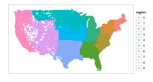
Now we wouldn’t be R users if we didn’t try to do something with data, even if it’s just a lookup table of zip codes. So let’s take a look at how they’re distributed by first digit:

library(zipcode)
library(ggplot2)

data(zipcode)
zipcode$region = substr(zipcode$zip, 1, 1)

g = ggplot(data=zipcode) + geom_point(aes(x=longitude, y=latitude, colour=region))

# simplify display and limit to the "lower 48"
g = g + theme_bw() + scale_x_continuous(limits = c(-125,-66), breaks = NA)
g = g + scale_y_continuous(limits = c(25,50), breaks = NA)

# don't need axis labels
g = g + labs(x=NULL, y=NULL)

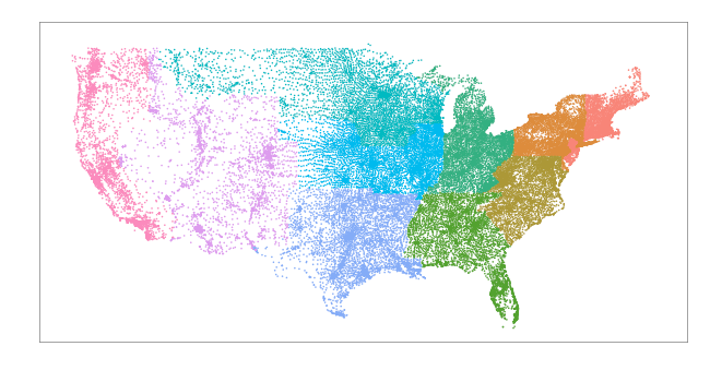
If we make the points smaller, cities and interstates are clearly visible, at least once you leave the Northeast Megalopolis:

how to install 64-bit rggobi on Mac OS X 10.5

I was surprised when everything seemed to “just work” when I made the jump to 64-bit R 2.11.1 a while back. “Surprised” because my previous attempt to join the 64-bit world under 2.10.x was a dead-end: the must-have RMySQL package didn’t like the 32-bit MySQL drivers, but Leopard’s 32-bit perl couldn’t deal with 64-bit drivers, etc., etc. Too much hassle for my new non-IT self to deal with.

So today I found the first thing which didn’t “just work” in the jump: the rggobi package.

Long story short, the trick is to install the rggobi package from source. Hadley Wickham (that guy is everywhere, isn’t he?) spells out the prerequisites and steps on the GGobi users Google group:

http://groups.google.com/group/ggobi/msg/5ae98c8b87d14a61

The only change you’ll need to make, if you’re still stuck in the 32/64-bit limbo of 10.5 like me is to make sure you build the package from the 64-bit version of R:

$ R64 CMD INSTALL ~/Downloads/rggobi_2.1.16.tar.gz

Posted in Tips. Tags: , , . Leave a Comment »

Incremental improvements to Nightlights mapping thanks to R-Bloggers

My recent post Nightlights: cool data, bad geocoding highlighted some of the geocoding challenges Steve Mosher has been finding as he works with this interesting “light pollution” data set.

It was also my first article reposted on Tal Galili’s fantastic R-Bloggers site which I have been following for a while. But even better than the surge of new visitors were the great comments and suggestions posted by members of the community. In this post, I’m going to walk through each suggestion to illustrate just how generous and helpful this community can be.

Our starting point is where we ended up in my first post, using ggplot2 to display the raster nightlights data and map overlay:

library(RCurl)
library(R.utils)
library(rgdal)
library(raster)

url_radianceCalibrated = "ftp://ftp.ngdc.noaa.gov/DMSP/web_data/x_rad_cal/rad_cal.tar"
calibratedLights = "rad_cal.tar"
hiResTif = "world_avg.tif"

download.file(url_radianceCalibrated,calibratedLights,mode="wb")
untar(calibratedLights)
gunzip( paste(hiResTif, '.gz', sep='') )

hiResLights = raster( hiResTif )

# Eastern Mass., Cape Cod & Islands:
e = extent(-71.5, -69.5, 41, 43)

r = crop(hiResLights,e)
p = rasterToPoints(r)
df = data.frame(p)
colnames(df) = c("lon", "lat", "dn")

g = ggplot( data=df) + geom_point(aes(x=lon, y=lat, color=dn) )
g = g + scale_colour_gradient(low="black", high="white", trans="sqrt")
g = g + theme_bw() + xlim(c(-71.5,-69.5)) + ylim(c(41,43))
g = g + opts( axis.text.x = theme_blank(), axis.text.y = theme_blank() )
g = g + borders("state", colour="yellow", alpha=0.5)

Note the mismatch between the data and map overlay and the weirdness in the map where points are missing on the North Shore:

original data, positioning, and borders in ggplot2

Ben Bolker suggested a way to eliminate the artifacts which led me to this discussion on R-sig-Geo between Hadley Wickham and Paul Hiemstra which tipped me off to the existence of geom_path layer in addition to the geom_polygon layer which borders() usually produces. Polygons are closed but paths need not be, so that helps. And ggplot2’s map_data() function seems to grab the same data as borders():

b = map_data("state")

g = ggplot( data=df) + geom_point(aes(x=lon, y=lat, color=dn) )
g = g + scale_colour_gradient(low="black", high="white", trans="sqrt")
g = g + theme_bw() + xlim(c(-71.5,-69.5)) + ylim(c(41,43))
g = g + opts( axis.text.x = theme_blank(), axis.text.y = theme_blank() )
g = g + geom_path(data=b, aes(x=long,y=lat,group=group), colour="yellow", alpha=0.5)

Bonus: geom_path() obeys the “alpha=0.5” directive to set the transparency:

Worst artifacts solved by switching to map_data() and geom_path()

But Robert Hijmans really hit it out the park with two great suggestions. First, he pointed me towards a much, much better source of coastline data by using raster’s getData() function to grab data from the GADM database of Global Administrative Areas:

usa = getData('GADM', country="USA", level=0)

Level 0 will get you country boundaries, Level 1 for state/province, and so on. So we’ll lose state boundaries, but these files are pretty big to start with and can take a lot longer to plot.

Also, be warned: apparently somebody sinned against The Church of GNU, so you may need to run gpclibPermit() manually before running fortify() on the SpatialPolygonsDataFrame:

> f_usa = fortify(usa)
Using GADMID to define regions.

	Note: polygon geometry computations in maptools
 	depend on the package gpclib, which has a
 	restricted licence. It is disabled by default;
 	to enable gpclib, type gpclibPermit()

Checking rgeos availability as gpclib substitute:
FALSE 
Error: isTRUE(gpclibPermitStatus()) is not TRUE
> gpclibPermit()
[1] TRUE

With that hoop cleared, we can fortify() and plot this new layer:

f_usa = fortify(usa)

g = ggplot( data=df) + geom_point(aes(x=lon, y=lat, color=dn) )
g = g + scale_colour_gradient(low="black", high="white", trans="sqrt")
g = g + theme_bw() + xlim(c(-71.5,-69.5)) + ylim(c(41,43))
g = g + opts( axis.text.x = theme_blank(), axis.text.y = theme_blank() )
g = g + geom_path(data=f_usa, aes(x=long,y=lat,group=group), colour="yellow", alpha=0.5)

The coordinates are still shifted, but—wow—what a beautiful coast line. Cape Ann on the North Shore is really there now:

beautiful coastline data from GADM

Robert also points out an important mismatch in that GDAL returns the top left corner and resolution, so we could be off by a pixel or so. A quick call to xmax() and ymax() will fix this in our original raster:

xmax(hiResLights) = 180
ymin(hiResLights) = -90

r = crop(hiResLights,e)
p = rasterToPoints(r)
df = data.frame(p)
colnames(df) = c("lon", "lat", "dn")

g = ggplot( data=df) + geom_point(aes(x=lon, y=lat, color=dn) )
g = g + scale_colour_gradient(low="black", high="white", trans="sqrt")
g = g + theme_bw() + xlim(c(-71.5,-69.5)) + ylim(c(41,43))
g = g + opts( axis.text.x = theme_blank(), axis.text.y = theme_blank() )
g = g + geom_path(data=f_usa, aes(x=long,y=lat,group=group), colour="yellow", alpha=0.5)

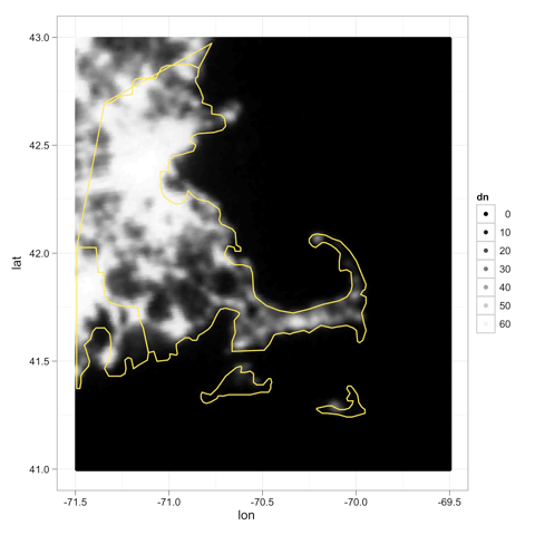
Hey, that’s not bad at all:

final try, after adjusting GDAL pixel shift

Looking at the final version leads me to wonder how much of the geocoding problem is position, and how much is resolution/blurring/smearing. The lights of Provincetown, for instance, look pretty good. Maybe the blob is too north by a few pixels, but at least it’s well contained by land now. On Nantucket, the blur is half in the harbor. Then again, on Nantucket, most of the lights are right on the harbor, from the ferry terminal and running east to main street. So the lights are just about where they should be. Perhaps they’re just blurred and therefore spill into the harbor?

But the real point of the post is to highlight the generosity of this community. For that, thanks. And again: welcome R-Bloggers readers!

vecLib: Why Mac users are better off with Open Source R

The July and August meetings of the New England R Users group focused on two different aspects of R performance: parallel processing techniques and the effects of compiler & library selection when compiling the R executable itself.

It was during Amy Szczepanski’s excellent introduction to multicore, Rmpi, and foreach (slides here) that she mentioned that the nice people who compile R for the Mac use optimized libraries to improve its performance. Amy works at the University of Tennessee’s Center for Remote Data Analysis and Visualization where they build and run machines with tens of thousands of cores, so her endorsement carries a lot of weight. I think Amy mentioned that she had benchmarked the open source vs. Revolutions distributions on her Mac, but I can’t find it in her slides and, well, in one ear and out the other….

It was the comprehensive presentation by IBM’s Vipin Sachdeva (slides here) showing 15-20X speedups through compiler and library selection that made me want to try a couple of benchmarks myself.  And my recent it’s-about-time upgrade to 2.11 seemed like the perfect opportunity.

Open source vs. Revolutions Community R

Performance is one of the advantages claimed by Revolution Analytics for its distributions, with their product page promising “optimized libraries and compiler techniques run most computation-intensive programs significantly faster than Base R” even with their free, Community edition. I have heard good things about its performance on Windows, so I was curious to see if it provides an improvement over the already-optimized Mac binary.

Benchmarking Methodology (or lack thereof)

First, some disclaimers: I am not a serious benchmarker and have made no special effort for statistical rigor.  I am just looking for order-of-magnitudes here, so I kept a normal number of programs running in the background, like Firefox and OpenOffice, though nothing was doing anything substantial and I avoided any user input while each test ran. My machine is the short-lived, late-2008, aluminum unibody 13″ MacBook (MacBook5,1) with 4GB RAM and Mac OS X Leopard 10.5.8 running the 32-bit kernel. It has a 2.4GHz Core 2 Duo — nothing special.

For my tests, I ran the standard R Benchmark 2.5 available from AT&T ‘s benchmarking page which performs various matrix and vector calculations — perfect for discerning the effects of such optimized libraries.  I kept the defaults, such as running each test 3 times, and installed the required “SuppDists” package.  I tested the open source 2.10.1 32-bit version I already had on my machine and then installed Revolution’s 2.10.1-based 64-bit community edition. I should have repeated the test with the open source 64-bit edition, but I didn’t think of it at the time (I told you I wasn’t serious about this), so instead I later re-ran the benchmark with the 32- and 64-bit versions of the open source 2.11.1 to check if there are any significant 32-vs-64 differences.

Results

It didn’t take long to realize that the Revolutions community edition was not going to fare well. During just the fourth benchmark, 2800×2800 cross-product matrix (b = a’ * a), there was a pregnant pause in the output while my laptop’s fans kicked in and soon spun up to full force. It took nearly 25 seconds to complete each turn of that one test where the open source 2.10.1 had finished in less than one tenth the time. (The complete output for each test is at the end of this post.)
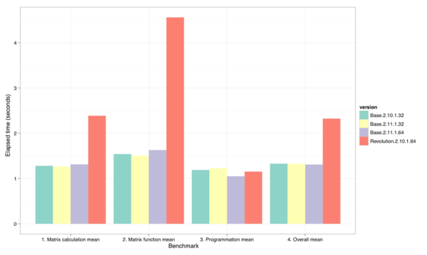
results summary bar chart

Figure 1: Summary-level benchmark results. (Smaller bars are better.)

Figure 1 shows the geometric means of the elapsed times for each benchmark section as reported by R Benchmark 2.5. Clearly the Revolutions distribution did significantly worse on the matrix benchmarks. Figure 2 drills into the individual benchmarks to show the roughly 2-8X difference on the five slowest matrix benchmarks. Only on the sixth, Grand common divisors of 400,000 pairs (recursion), was the slowdown matched by the base 64-bit distribution. Only on Revolution’s fastest benchmark,2400×2400 normal distributed random matrix ^1000 all the way at the bottom of Figure 2, did the 64-bit versions hold a distinct (and roughly equal) advantage over their 32-bit brethren.

results detail bar chart

Figure 2: Individual benchmark results. (Smaller bars are better.)

vecLib: BLAS, LAPACK, and built into the Mac

So, no surprise — Amy was right. The off-the-shelf open source distributions of R for the Mac are already optimized. But how? Vipin walked us through all the different choices for BLAS and LAPACK libraries, not to mention the different C and FORTRAN compilers and their optimization flags. How can we know what’s being used by a given distribution? Well, it turns out that R makes it easy to find out with the config options to “R CMD”:

$ R CMD config BLAS_LIBS-L/Library/Frameworks/R.framework/Resources/lib/i386 -lRblas
$ ls -l /Library/Frameworks/R.framework/Resources/lib/i386/libRblas.dylib
lrwxr-xr-x  1 root  admin  17 Oct  7 00:58 /Library/Frameworks/R.framework/Resources/lib/i386/libRblas.dylib -> ../libRblas.dylib
$ ls -l /Library/Frameworks/R.framework/Resources/lib/libRblas.dylib
lrwxr-xr-x  1 root  admin  21 Oct  7 00:58 /Library/Frameworks/R.framework/Resources/lib/libRblas.dylib -> libRblas.vecLib.dylib

Following the symbolic link, “libRblas.vecLib.dylib” is the library being used for BLAS. A quick consultation with Google reveals that “vecLib” is Apple’s vector library from their “Acceleration” framework in Mac OS. Here’s what Apple’s Developer site says about vecLib’s BLAS and LAPACK components::

Basic Linear Algebra Subprograms (BLAS)

VecLib also contains Basic Linear Algebra Subprograms (BLAS) that use AltiVec technology for their implementations. The functions are grouped into three categories (called levels), as follows:

  1. Vector-scalar linear algebra subprograms
  2. Matrix-vector linear algebra subprograms
  3. Matrix operations

A Readme file is included that contains the following sections:

  1. Descriptions of functions
  2. Comparison with BLAS (Basic Linear Algebra Subroutines)
  3. Test methodology
  4. Future releases
  5. Compiler version

LAPACK

LAPACK provides routines for solving systems of simultaneous linear equations, least-squares solutions of linear systems of equations, eigenvalue problems, and singular value problems. The associated matrix factorizations (LU, Cholesky, QR, SVD, Schur, generalized Schur) are also provided, as are related computations such as reordering of the Schur factorizations and estimating condition numbers. Dense and banded matrices are handled, but not general sparse matrices. In all areas, similar functionality is provided for real and complex matrices, in both single and double precision.

Also, see <http://netlib.org/lapack/index.html.

As Vipin had demonstrated, using a fast BLAS and LAPACK libraries can make all the difference in the world (well, 20X or so). And since Apple controls the horizontal and vertical on their platform, it shouldn’t be a surprise that vecLib is fast on their hardware and OS.  The real question is why doesn’t Revolutions simply link to vecLib too? It can’t be because their libraries are better (they clearly aren’t). Nor could they be afraid of competing with their Enterprise edition because, according to this edition comparison chart, they don’t offer an enterprise edition for the Mac. Perhaps they’re simply not that familiar with the platform and don’t know about vecLib. I know I didn’t know anything about it until these tests prompted me to consult The Google.

Your mileage may vary

Google also pointed me to this recent discussion on the R-SIG-MAC mailing list in which Simon Urbanek refers to a serious bug in vecLib which prevents it from spawning threads and shows timings from a “tcrossprod” benchmark on a new 2.66GHz Mac Pro:

vecLib           6.43
ATLAS serial     4.80
MKL serial       4.30
MKL parallel     0.90
ATLAS parallel   0.71

So there still seems to be plenty of opportunity to beat vecLib if you’re willing to compile R and mix and match BLAS libraries. For the rest of us, the open source distribution offers the best bang for the buck.

Maybe I need to ask Vipin to take a look at my Mac at the next meeting….

Complete Output

open source 2.10.1 32-bit

R version 2.10.1 (2009-12-14)
Copyright (C) 2009 The R Foundation for Statistical Computing
ISBN 3-900051-07-0

R is free software and comes with ABSOLUTELY NO WARRANTY.
You are welcome to redistribute it under certain conditions.
Type 'license()' or 'licence()' for distribution details.

 Natural language support but running in an English locale

R is a collaborative project with many contributors.
Type 'contributors()' for more information and
'citation()' on how to cite R or R packages in publications.

Type 'demo()' for some demos, 'help()' for on-line help, or
'help.start()' for an HTML browser interface to help.
Type 'q()' to quit R.

[R.app GUI 1.31 (5537) i386-apple-darwin8.11.1]

[Workspace restored from /Users/jbreen/.RData]

> source("/Users/jbreen/Desktop/R-benchmark-25.R")
Loading required package: Matrix
Loading required package: lattice
Loading required package: SuppDists

 R Benchmark 2.5
 ===============
Number of times each test is run__________________________:  3

 I. Matrix calculation
 ---------------------
Creation, transp., deformation of a 2500x2500 matrix (sec):  1.16766666666666
2400x2400 normal distributed random matrix ^1000____ (sec):  1.14666666666667
Sorting of 7,000,000 random values__________________ (sec):  1.26266666666667
2800x2800 cross-product matrix (b = a' * a)_________ (sec):  2.461
Linear regr. over a 3000x3000 matrix (c = a \ b')___ (sec):  1.42233333333333
 --------------------------------------------
 Trimmed geom. mean (2 extremes eliminated):  1.27997944504873

 II. Matrix functions
 --------------------
FFT over 2,400,000 random values____________________ (sec):  1.333
Eigenvalues of a 640x640 random matrix______________ (sec):  1.23633333333333
Determinant of a 2500x2500 random matrix____________ (sec):  1.65233333333333
Cholesky decomposition of a 3000x3000 matrix________ (sec):  1.712
Inverse of a 1600x1600 random matrix________________ (sec):  1.65633333333334
 --------------------------------------------
 Trimmed geom. mean (2 extremes eliminated):  1.53942494113224

 III. Programmation
 ------------------
3,500,000 Fibonacci numbers calculation (vector calc)(sec):  1.21066666666667
Creation of a 3000x3000 Hilbert matrix (matrix calc) (sec):  0.919333333333332
Grand common divisors of 400,000 pairs (recursion)__ (sec):  1.252
Creation of a 500x500 Toeplitz matrix (loops)_______ (sec):  1.38000000000001
Escoufier's method on a 45x45 matrix (mixed)________ (sec):  1.105
 --------------------------------------------
 Trimmed geom. mean (2 extremes eliminated):  1.18758233972606

Total time for all 15 tests_________________________ (sec):  20.9173333333333
Overall mean (sum of I, II and III trimmed means/3)_ (sec):  1.32762395973868
 --- End of test ---

Revolution R community 2.10.1 64 bit

R version 2.10.1 (2009-12-14)
Copyright (C) 2009 The R Foundation for Statistical Computing
ISBN 3-900051-07-0

R is free software and comes with ABSOLUTELY NO WARRANTY.
You are welcome to redistribute it under certain conditions.
Type 'license()' or 'licence()' for distribution details.

R is a collaborative project with many contributors.
Type 'contributors()' for more information and
'citation()' on how to cite R or R packages in publications.

Type 'demo()' for some demos, 'help()' for on-line help, or
'help.start()' for an HTML browser interface to help.
Type 'q()' to quit R.

REvolution R version 3.2: an enhanced distribution of R
REvolution Computing packages Copyright (C) 2010 REvolution Computing, Inc.

Type 'revo()' to visit www.revolution-computing.com for the latest
REvolution R news, 'forum()' for the community forum, or 'readme()'
for release notes.

[R.app GUI 1.30 (5511) x86_64-apple-darwin9.8.0]

[Workspace restored from /Users/jbreen/.RData]

trying URL 'http://watson.nci.nih.gov/cran_mirror/src/contrib/SuppDists_1.1-8.tar.gz'
Content type 'application/x-gzip' length 139864 bytes (136 Kb)
opened URL
==================================================
downloaded 136 Kb

* installing *source* package ‘SuppDists’ ...
** libs
** arch - x86_64
g++ -arch x86_64  -I/opt/REvolution/Revo-3.2/Revo64/R.framework/Resources/include -I/opt/REvolution/Revo-3.2/Revo64/R.framework/Resources/include/x86_64  -I/usr/local/include    -fPIC  -g -O2 -c dists.cc -o dists.o
g++ -arch x86_64 -dynamiclib -Wl,-headerpad_max_install_names -undefined dynamic_lookup -single_module -multiply_defined suppress -L/usr/local/lib -o SuppDists.so dists.o -F/opt/REvolution/Revo-3.2/Revo64/R.framework/.. -framework R -Wl,-framework -Wl,CoreFoundation
** R
** preparing package for lazy loading
** help
*** installing help indices
** building package indices ...
* DONE (SuppDists)

The downloaded packages are in
 ‘/private/var/folders/+s/+snLnQILHz4Kn8jMFYEERE++-4+/-Tmp-/RtmpVqNN4f/downloaded_packages’
> source("/Users/jbreen/Desktop/R-benchmark-25.R")
Loading required package: Matrix
Loading required package: lattice
Loading required package: SuppDists

 R Benchmark 2.5
 ===============
Number of times each test is run__________________________:  3

 I. Matrix calculation
 ---------------------
Creation, transp., deformation of a 2500x2500 matrix (sec):  1.18633333333333
2400x2400 normal distributed random matrix ^1000____ (sec):  0.463333333333334
Sorting of 7,000,000 random values__________________ (sec):  1.10266666666667
2800x2800 cross-product matrix (b = a' * a)_________ (sec):  24.786
Linear regr. over a 3000x3000 matrix (c = a \ b')___ (sec):  10.3813333333333
 --------------------------------------------
 Trimmed geom. mean (2 extremes eliminated):  2.38580368558367

 II. Matrix functions
 --------------------
FFT over 2,400,000 random values____________________ (sec):  1.32633333333335
Eigenvalues of a 640x640 random matrix______________ (sec):  1.631
Determinant of a 2500x2500 random matrix____________ (sec):  8.66366666666666
Cholesky decomposition of a 3000x3000 matrix________ (sec):  6.70300000000001
Inverse of a 1600x1600 random matrix________________ (sec):  8.71566666666664
 --------------------------------------------
 Trimmed geom. mean (2 extremes eliminated):  4.55835668372464

 III. Programmation
 ------------------
3,500,000 Fibonacci numbers calculation (vector calc)(sec):  1.10766666666666
Creation of a 3000x3000 Hilbert matrix (matrix calc) (sec):  0.818666666666672
Grand common divisors of 400,000 pairs (recursion)__ (sec):  3.529
Creation of a 500x500 Toeplitz matrix (loops)_______ (sec):  1.28933333333335
Escoufier's method on a 45x45 matrix (mixed)________ (sec):  1.072
 --------------------------------------------
 Trimmed geom. mean (2 extremes eliminated):  1.15254093929808

Total time for all 15 tests_________________________ (sec):  72.776
Overall mean (sum of I, II and III trimmed means/3)_ (sec):  2.32291395838888
 --- End of test ---

open source 2.11.1 64-bit

R version 2.11.1 (2010-05-31)
Copyright (C) 2010 The R Foundation for Statistical Computing
ISBN 3-900051-07-0

R is free software and comes with ABSOLUTELY NO WARRANTY.
You are welcome to redistribute it under certain conditions.
Type 'license()' or 'licence()' for distribution details.

 Natural language support but running in an English locale

R is a collaborative project with many contributors.
Type 'contributors()' for more information and
'citation()' on how to cite R or R packages in publications.

Type 'demo()' for some demos, 'help()' for on-line help, or
'help.start()' for an HTML browser interface to help.
Type 'q()' to quit R.

[R.app GUI 1.34 (5589) x86_64-apple-darwin9.8.0]

[Workspace restored from /Users/jbreen/.RData]

> source("/Users/jbreen/Desktop/R-benchmark-25.R")
Loading required package: Matrix
Loading required package: lattice

Attaching package: 'Matrix'

The following object(s) are masked from 'package:base':

 det

Loading required package: SuppDists
Error in eval.with.vis(expr, envir, enclos) : object 'rMWC1019' not found
In addition: Warning message:
In library(package, lib.loc = lib.loc, character.only = TRUE, logical.return = TRUE,  :
 there is no package called 'SuppDists'
trying URL 'http://watson.nci.nih.gov/cran_mirror/bin/macosx/leopard/contrib/2.11/SuppDists_1.1-8.tgz'
Content type 'application/x-gzip' length 412485 bytes (402 Kb)
opened URL
==================================================
downloaded 402 Kb

The downloaded packages are in
 /var/folders/+s/+snLnQILHz4Kn8jMFYEERE++-4+/-Tmp-//RtmpoWgMNZ/downloaded_packages
> source("/Users/jbreen/Desktop/R-benchmark-25.R")
Loading required package: SuppDists

 R Benchmark 2.5
 ===============
Number of times each test is run__________________________:  3

 I. Matrix calculation
 ---------------------
Creation, transp., deformation of a 2500x2500 matrix (sec):  1.193
2400x2400 normal distributed random matrix ^1000____ (sec):  0.455333333333336
Sorting of 7,000,000 random values__________________ (sec):  1.06133333333333
2800x2800 cross-product matrix (b = a' * a)_________ (sec):  2.70466666666667
Linear regr. over a 3000x3000 matrix (c = a \ b')___ (sec):  1.78500000000001
 --------------------------------------------
 Trimmed geom. mean (2 extremes eliminated):  1.3123313069964

 II. Matrix functions
 --------------------
FFT over 2,400,000 random values____________________ (sec):  1.23466666666667
Eigenvalues of a 640x640 random matrix______________ (sec):  1.15366666666667
Determinant of a 2500x2500 random matrix____________ (sec):  1.92633333333333
Cholesky decomposition of a 3000x3000 matrix________ (sec):  1.81366666666667
Inverse of a 1600x1600 random matrix________________ (sec):  1.96333333333333
 --------------------------------------------
 Trimmed geom. mean (2 extremes eliminated):  1.6278443559224

 III. Programmation
 ------------------
3,500,000 Fibonacci numbers calculation (vector calc)(sec):  1.07533333333332
Creation of a 3000x3000 Hilbert matrix (matrix calc) (sec):  0.792999999999997
Grand common divisors of 400,000 pairs (recursion)__ (sec):  3.393
Creation of a 500x500 Toeplitz matrix (loops)_______ (sec):  1.20000000000001
Escoufier's method on a 45x45 matrix (mixed)________ (sec):  0.89500000000001
 --------------------------------------------
 Trimmed geom. mean (2 extremes eliminated):  1.04917789012305

Total time for all 15 tests_________________________ (sec):  22.6473333333333
Overall mean (sum of I, II and III trimmed means/3)_ (sec):  1.30868512419174
 --- End of test ---

open source 2.11.1 32 bit

R version 2.11.1 (2010-05-31)
Copyright (C) 2010 The R Foundation for Statistical Computing
ISBN 3-900051-07-0

R is free software and comes with ABSOLUTELY NO WARRANTY.
You are welcome to redistribute it under certain conditions.
Type 'license()' or 'licence()' for distribution details.

 Natural language support but running in an English locale

R is a collaborative project with many contributors.
Type 'contributors()' for more information and
'citation()' on how to cite R or R packages in publications.

Type 'demo()' for some demos, 'help()' for on-line help, or
'help.start()' for an HTML browser interface to help.
Type 'q()' to quit R.

[R.app GUI 1.34 (5589) i386-apple-darwin9.8.0]

[Workspace restored from /Users/jbreen/.RData]

trying URL 'http://watson.nci.nih.gov/cran_mirror/bin/macosx/leopard/contrib/2.11/SuppDists_1.1-8.tgz'
Content type 'application/x-gzip' length 412485 bytes (402 Kb)
opened URL
==================================================
downloaded 402 Kb

The downloaded packages are in
 /var/folders/+s/+snLnQILHz4Kn8jMFYEERE++-4+/-Tmp-//RtmpX3gq6O/downloaded_packages
> source("/Users/jbreen/Desktop/R-benchmark-25.R")
Loading required package: Matrix
Loading required package: lattice

Attaching package: 'Matrix'

The following object(s) are masked from 'package:base':

 det

Loading required package: SuppDists

 R Benchmark 2.5
 ===============
Number of times each test is run__________________________:  3

 I. Matrix calculation
 ---------------------
Creation, transp., deformation of a 2500x2500 matrix (sec):  1.19433333333333
2400x2400 normal distributed random matrix ^1000____ (sec):  1.122
Sorting of 7,000,000 random values__________________ (sec):  1.144
2800x2800 cross-product matrix (b = a' * a)_________ (sec):  2.25133333333333
Linear regr. over a 3000x3000 matrix (c = a \ b')___ (sec):  1.475
 --------------------------------------------
 Trimmed geom. mean (2 extremes eliminated):  1.26312946510292

 II. Matrix functions
 --------------------
FFT over 2,400,000 random values____________________ (sec):  1.40366666666667
Eigenvalues of a 640x640 random matrix______________ (sec):  1.28133333333333
Determinant of a 2500x2500 random matrix____________ (sec):  1.745
Cholesky decomposition of a 3000x3000 matrix________ (sec):  1.61
Inverse of a 1600x1600 random matrix________________ (sec):  1.50166666666667
 --------------------------------------------
 Trimmed geom. mean (2 extremes eliminated):  1.50275368328927

 III. Programmation
 ------------------
3,500,000 Fibonacci numbers calculation (vector calc)(sec):  1.22666666666666
Creation of a 3000x3000 Hilbert matrix (matrix calc) (sec):  0.87133333333333
Grand common divisors of 400,000 pairs (recursion)__ (sec):  1.29
Creation of a 500x500 Toeplitz matrix (loops)_______ (sec):  1.33899999999999
Escoufier's method on a 45x45 matrix (mixed)________ (sec):  1.16800000000001
 --------------------------------------------
 Trimmed geom. mean (2 extremes eliminated):  1.22721231763175

Total time for all 15 tests_________________________ (sec):  20.6233333333333
Overall mean (sum of I, II and III trimmed means/3)_ (sec):  1.32561819861344
 --- End of test ---
Posted in Tips. Tags: , , . 5 Comments »

Nightlights: cool data, bad geocoding

A global source of population density has been on my low-priority wish list for some time, so I was very excited when I found Steve Mosher’s work with the Nighlights data set. “Nightlights” refers to the artificial lights seen from space at night. Astronomers call it “light pollution” which is pretty accurate since it’s decidedly not the light which we all use to see and avoid peril at night. Rather, it’s the light (and energy) wasted in that pursuit by being emitted or reflected straight up into the sky.

Steve has since spent some quality time with other R packages like Rgooglemap exploring this data set and has noticed some problems with the geocoding of the nightlights data.  I noticed the same thing, though much more naively, just trying to check out the data around my home:

library(RCurl)
library(R.utils)
library(rgdal)
library(raster)

url_radianceCalibrated = "ftp://ftp.ngdc.noaa.gov/DMSP/web_data/x_rad_cal/rad_cal.tar"
calibratedLights = "rad_cal.tar"
hiResTif = "world_avg.tif"

download.file(url_radianceCalibrated,calibratedLights,mode="wb")
untar(calibratedLights)
gunzip(paste(hiResTif, '.gz', sep='')

hiResLights = raster("world_avg.tif")

# Eastern Mass., Cape Cod & Islands:
e = extent(-71.5, -69.5, 41, 43)

r = crop(hiResLights,e)
plot(r)

which looks amazing… right up until you overlay the county boundaries from the standard ‘maps’ package:

library(maps)
map("county",xlim=c(-71.5,-69.5),ylim=c(41,43),add=T)

Alas. To my eye, there’s a clear shift to the northwest (see Provincetown at the tip of Cape Cod), and perhaps a bit of a clockwise rotation as well (see the big bulge of Cape Ann north of Boston).

Newer = better… ?

I have a lot to learn about this data, but in my poking around, I did find more recent observations available on a “Version 4 DMSP-OLS Nighttime Lights Time Series” page. But warning — these files are big. The tar file I download next is over 350MB:

url = "http://www.ngdc.noaa.gov/dmsp/data/web_data/v4composites/F152007.v4.tar"
dest = "F152007.v4.tar"
tif = "F152007.v4b_web.stable_lights.avg_vis.tif"

download.file(url, dest)
untar(dest)
gunzip( paste(tif, '.gz', sep='') )

f15 = raster(tif)
e = extent(-71.5, -69.5, 41, 43)
r = crop(f15, e)
plot(r)
map("county",xlim=c(-71.5,-69.5),ylim=c(41,43),add=T)

which looks a lot better, though still probably not perfect.

ggplot2 with raster

I am a huge fan of ggplot2, but since this was my first exposure to the raster package, I just copied and pasted Steve’s code to make the plots. But I couldn’t help myself to try to reproduce them in ggplot2.

Getting your data into a data.frame is the key to using ggplot2. Fortunately, the raster package includes a rasterToPoints() function which outputs a list which is easily cast to a data.frame:

p = rasterToPoints(r)
df = data.frame(p)
colnames(df) = c("lon", "lat", "dn")

which makes the actual plotting so easy, even qplot() will do it:

library(ggplot2)
qplot(lon, lat, color=dn, data=df) 
  + scale_colour_gradient(low="black", high='white', transform='sqrt') 
  + theme_bw() + borders("state", colour="yellow") 
  + xlim(c(-71.5, -69.5)) + ylim(c(41, 43))

The only technical glitch is in the overlay, as zooming in truncates the northernmost coastline points but the geom_polygon() layer created by borders() seems compelled to close the shape and connects the northern Mass. coast with Rhode Island.

rgdal and other GIS-related packages for Mac OS X

CRAN contains ready-made binary packages for nearly all of its packages, but rgdal is one which I keep finding myself trying to install from source whenever I upgrade R.

Compiled versions of rgdal, along with prerequisites and complements like the GDAL framework, GRASS, and even the old FFTW3 can be found at KyngChaos’s Wiki:


Update 10/10/10:
I don’t remember needing to do this before, but

$ ln -s /Library/Frameworks/GDAL.framework/Programs/gdal-config /usr/local/bin

makes the rgdal source package installation work on R 2.11.1.


Posted in GIS, Tips. Tags: , , . Leave a Comment »