slides from my R tutorial on Twitter text mining #rstats

Update: An expanded version of this tutorial will appear in the new Elsevier book Practical Text Mining and Statistical Analysis for Non-structured Text Data Applications by Gary Miner et. al which is now available for pre-order from Amazon.

In conjunction with the book, I have cleaned up the tutorial code and published it on github.


Last month I presented this introduction to R at the Boston Predictive Analytics MeetUp on Twitter Sentiment.

The goal of the presentation was to expose a first-time (but technically savvy) audience to working in R. The scenario we work through is to estimate the sentiment expressed in tweets about major U.S. airlines. Even with a tiny sample and a very crude algorithm (simply counting the number of positive vs. negative words), we find a believable result. We conclude by comparing our result with scores we scrape from the American Consumer Satisfaction Index web site.

Jeff Gentry’s twitteR package makes it easy to fetch the tweets. Also featured are the plyr, ggplot2, doBy, and XML packages. A real analysis would, no doubt, lean heavily on the tm text mining package for stemming, etc.

Here is the slimmed-down version of the slides:

And here’s a PDF version to download.

Special thanks to John Verostek for putting together such an interesting event, and for providing valuable feedback and help with these slides.


Update: thanks to eagle-eyed Carl Howe for noticing a slightly out-of-date version of the score.sentiment() function in the deck. Missing was handling for NA values from match(). The deck has been updated and the code is reproduced here for convenience:


score.sentiment = function(sentences, pos.words, neg.words, .progress='none')
{
	require(plyr)
	require(stringr)
	
	# we got a vector of sentences. plyr will handle a list
	# or a vector as an "l" for us
	# we want a simple array ("a") of scores back, so we use 
	# "l" + "a" + "ply" = "laply":
	scores = laply(sentences, function(sentence, pos.words, neg.words) {
		
		# clean up sentences with R's regex-driven global substitute, gsub():
		sentence = gsub('[[:punct:]]', '', sentence)
		sentence = gsub('[[:cntrl:]]', '', sentence)
		sentence = gsub('\\d+', '', sentence)
		# and convert to lower case:
		sentence = tolower(sentence)

		# split into words. str_split is in the stringr package
		word.list = str_split(sentence, '\\s+')
		# sometimes a list() is one level of hierarchy too much
		words = unlist(word.list)

		# compare our words to the dictionaries of positive & negative terms
		pos.matches = match(words, pos.words)
		neg.matches = match(words, neg.words)
	
		# match() returns the position of the matched term or NA
		# we just want a TRUE/FALSE:
		pos.matches = !is.na(pos.matches)
		neg.matches = !is.na(neg.matches)

		# and conveniently enough, TRUE/FALSE will be treated as 1/0 by sum():
		score = sum(pos.matches) - sum(neg.matches)

		return(score)
	}, pos.words, neg.words, .progress=.progress )

	scores.df = data.frame(score=scores, text=sentences)
	return(scores.df)
}

Hype isn’t limited to IT vendors: presenting my new Turbo Force High Velocity Circulator

I went to the store to purchase a small fan to blow nice cool air towards my desk. But when I got it home and took a closer look, it turns out that I had selected an HT-900 Turbo Force® Air Circulator Fan from Honeywell.

Honeywell, eh? They make jet engines and ammonium nitrate fertilizer which won’t blow up! Maybe there’s more to this fan than I realized.

Intruiged, I started to read the Owner’s Manual:

The Turbo Force® High Velocity Air Circulator Fans are aerodynamically designed to give you the versatility of changing this fan’s angular direction simply by adjusting the fan to ANY desired angular output (Fig.1).

I think that means: It tilts.

The introduction continues:

Upon using this fan, you will feel a strong and powerful air stream that will quickly move air in order to cool an area rapidly and efficiently.

Translation: Turn it on and it will blow air.

Suddenly all that vendor verbiage about how cloud computing will increase the synergies between your technology and business priorities sounds… well… not that bad. At least they’re not hyping something as simple as a desk fan.

googleVis-0.2.4 requires older version of RJSONIO (0.5-0) #rstats

[Update: the new release of googleVis accounts for changes in RJSONIO’s handling of backslashes, so you probably won’t need the older version.]

Something has apparently changed in the way RJSON’s toJSON() function works which is causing all sorts of extra escape characters (backslashes) to appear in the googleVis-generated JavaScript, at least when trying to set a visualization’s initial state. This bogus code causes the browser’s JavaScript engine to choke just before it can call chart.draw(), so you don’t see the Flash visualization at all–just a blank space with the pretty footer.

This is at least the case on Mac OS 10.6.7 and Markus Gesmann gets all the credit for tracking it down.

Here’s an example state string which selects a couple of bubbles to be labeled (“Oranges” and “Apples”) and sets the time to start about half-way through:

state.json='{"xAxisOption":"3","xZoomedDataMin":81,"playDuration":15000,"sizeOption":"_UNISIZE","xZoomedDataMax":111,"xLambda":1,"dimensions":{"iconDimensions":["dim0"]},"yZoomedDataMax":91,"duration":{"multiplier":1,"timeUnit":"Y"},"orderedByX":false,"xZoomedIn":false,"yZoomedDataMin":71,"showTrails":false,"orderedByY":false,"iconType":"BUBBLE","uniColorForNonSelected":false,"yZoomedIn":false,"nonSelectedAlpha":0.4,"yLambda":1,"time":"2010","yAxisOption":"4","iconKeySettings":[{"LabelY":27,"key":{"dim0":"Apples"},"LabelX":42}],"colorOption":"6"}'

# create the motion chart
M=gvisMotionChart(Fruits, "Fruit", "Year", options=list(state=state.json))

Here’s the output in question using the current RJSONIO 0.7:

> cat(M$html$chart['jsDrawChart'])

// jsDrawChart
function drawChartMotionChartID6db280db() {
  var data = gvisDataMotionChartID6db280db()
  var chart = new google.visualization.MotionChart(
   document.getElementById('MotionChartID6db280db')
  );
  var options ={};
options["width"] = [    600 ];
options["height"] = [    500 ];
options["state"] = [ "{\\"xAxisOption\\":\\"3\\",\\"xZoomedDataMin\\":81,\\"playDuration\\":15000,\\"sizeOption\\":\\"_UNISIZE\\",\\"xZoomedDataMax\\":111,\\"xLambda\\":1,\\"dimensions\\":{\\"iconDimensions\\":[\\"dim0\\"]},\\"yZoomedDataMax\\":91,\\"duration\\":{\\"multiplier\\":1,\\"timeUnit\\":\\"Y\\"},\\"orderedByX\\":false,\\"xZoomedIn\\":false,\\"yZoomedDataMin\\":71,\\"showTrails\\":false,\\"orderedByY\\":false,\\"iconType\\":\\"BUBBLE\\",\\"uniColorForNonSelected\\":false,\\"yZoomedIn\\":false,\\"nonSelectedAlpha\\":0.4,\\"yLambda\\":1,\\"time\\":\\"2010\\",\\"yAxisOption\\":\\"4\\",\\"iconKeySettings\\":[{\\"LabelY\\":27,\\"key\\":{\\"dim0\\":\\"Apples\\"},\\"LabelX\\":42}],\\"colorOption\\":\\"6\\"}" ];
  chart.draw(data,options);
}

And here’s working code from RJSONIO 0.5:

> cat(M$html$chart['jsDrawChart'])

// jsDrawChart
function drawChartMotionChartID47a55df7() {
  var data = gvisDataMotionChartID47a55df7()
  var chart = new google.visualization.MotionChart(
   document.getElementById('MotionChartID47a55df7')
  );
  var options ={};
options["width"] =    600;
options["height"] =    500;
options["state"] = "{\"sizeOption\":\"5\",\"nonSelectedAlpha\":0.4,\"xLambda\":1,\"iconType\":\"BUBBLE\",\"yZoomedDataMax\":91,\"iconKeySettings\":[{\"LabelY\":-124,\"LabelX\":-160,\"key\":{\"dim0\":\"Oranges\"}},{\"LabelY\":53,\"LabelX\":37,\"key\":{\"dim0\":\"Apples\"}}],\"xZoomedIn\":false,\"orderedByX\":false,\"showTrails\":false,\"yZoomedIn\":false,\"yZoomedDataMin\":71,\"xZoomedDataMin\":81,\"orderedByY\":false,\"xAxisOption\":\"3\",\"yAxisOption\":\"4\",\"uniColorForNonSelected\":false,\"duration\":{\"timeUnit\":\"Y\",\"multiplier\":1},\"time\":\"2009\",\"yLambda\":1,\"xZoomedDataMax\":111,\"dimensions\":{\"iconDimensions\":[\"dim0\"]},\"colorOption\":\"2\",\"playDuration\":15000}";
  chart.draw(data,options);
}

Maybe this post can help others avoid the blank look I had on my face as I kept staring at a blank page in my browser.

quantmod makes it easy to watch silver prices crash in R #rstats

As if there hasn’t been enough going on this week, silver prices have fallen nearly $10 per ounce. That’s a reduction of over 20%. Jeffrey Ryan’s quantmod package makes it easy to download the latest prices from OANDA’s web site and plot the excitement.

The getSymbols() function is at the heart of quantmod’s data retrieval prowess, currently handling Yahoo! Finance, Google Finance, the St. Louis Fed’s FRED, and OANDA sites, in addition to MySQL databases and RData and CSV files.

First a word of warning: if you have a computer science background, you may cringe at the way getSymbols() returns data. Rather than returning the fetched data as the result of a function call, it populates your R session’s .GlobalEnv environment (or another one of your choosing via the env parameter) with xts and zoo objects containing your data. For example, if you ask for IBM’s stock prices via getSymbols("IBM"), you will find the data in a new “IBM” object in your .GlobalEnv. This behavior can be changed by setting auto.assign=F, but then you can only request one symbol at a time. But this is a minor nit about an incredibly useful package.

There’s even a wrapper function to help retrieve precious metal prices, and we will use this getMetals() function to retrieve the last year’s worth of prices for gold (XAU) and silver (XAG):

library(quantmod)
getMetals(c('XAU', 'XAG'), from=Sys.Date()-365)

Yup — that’s it. getMetals() lets us know it has created two new objects:

[1] "XAUUSD" "XAGUSD"

There were also few warning messages complaining about the last line in the downloaded file. I haven’t bothered to dig into it as the data seem fine, including today’s price:

> ls()
[1] "XAGUSD" "XAUUSD"

> head(XAGUSD)
           XAG.USD
2010-05-07 17.6600
2010-05-08 18.4600
2010-05-09 18.4320
2010-05-10 18.4336
2010-05-11 18.5400
2010-05-12 19.3300

> tail(XAGUSD)
           XAG.USD
2011-05-02 47.9850
2011-05-03 45.2373
2011-05-04 44.0238
2011-05-05 40.9171
2011-05-06 37.9939
2011-05-07 35.0598

And here’s how easy it is to use the package’s built-in graphing facilities:

chartSeries(XAUUSD, theme="white")

chartSeries(XAGUSD, theme="white")

Yup — that’s quite a shellacking for silver.

Now I tend to be a ggplot2 guy myself, and I have never actually worked with xts or zoo objects before, but it’s pretty easy to get them into a suitable data.frame:

silver = data.frame(XAGUSD)
silver$date = as.Date(rownames(silver))
colnames(silver)[1] = 'price'

library(ggplot2)
ggplot(data=silver, aes(x=date, y=price)) + geom_line() + theme_bw()

Slides: “Accessing Databases from R” #rstats

For the past few meetings of the Greater Boston useR Group, we have been opened with an introductory “useR Vignette” talk on a topic which may be helpful for new R users. This week, I presented an overview of accessing databases from R. Several people have tweeted and blogged nice things about my talk
and have asked for the slides, so here they are, via Slideshare:

The final slide includes the code which I used to create and populate the ‘testdb’ database I used for my examples. I have duplicated it here as it’s a nice, quick example of using DBI to store an R data.frame in a database:

First, create new database & user in MySQL:

mysql> create database testdb;
mysql> grant all privileges on testdb.* to 'testuser'@'localhost' identified by 'testpass';
mysql> flush privileges;

In R, load the “mtcars” data.frame, clean it up, and write it to a new “motortrend” table:

library(stringr)
library(RMySQL)

data(mtcars)

# car name is data.frame's rownames. Let's split into manufacturer and model columns:
mtcars$mfg = str_split_fixed(rownames(mtcars), ' ', 2)[,1]
mtcars$mfg[mtcars$mfg=='Merc'] = 'Mercedes'
mtcars$model = str_split_fixed(rownames(mtcars), ' ', 2)[,2]

# connect to local MySQL database (host='localhost' by default)
con = dbConnect("MySQL", "testdb", username="testuser", password="testpass")

dbWriteTable(con, 'motortrend', mtcars)

dbDisconnect(con)

4 lines of R to get you started using the Rook web server interface

Now that Jeffrey Horner has settled on a name for his new package… the Rook web server interface is now available on CRAN.

Rook provides an interface for R programmers to build web applications which can run in R 2.13’s built-in web server or (soon) rApache.

Jeffrey’s provided some great documentation and sample code on his blog, in the README file, and in the package documentation itself, but somehow I completely missed the importance of the Rhttpd class and couldn’t figure out how to load or launch any of the examples.

Hopefully I can save someone some similar head-scratching. The key is the Rhttpd class, which controls the web server and manages applications. By default it will install the “RookTest” example, so here are 4 lines you need to see it work:

> library(Rook)
> s <- Rhttpd$new()
> s$start(quiet=TRUE)
> s$print()

Server started on 127.0.0.1:31839
[1] RookTest http://127.0.0.1:31839/custom/RookTest

Call browse() with an index number or name to run an application.

[EDIT: Thanks to Jim Porzak to pointing out that browse() is a method on the Rhttpd object rather than an old school package-scoped function. Times are a-changin’… for the better!]

The browse() function didn’t seem to work for me, s$browse(1) will load the URL into your browser or you can just copy-and-paste to access the running application:

Enjoy!

Posted in Tips. Tags: , . 11 Comments »

Abusing Amazon’s Elastic MapReduce Hadoop service… easily, from R

I built my first Hadoop cluster this week and ran my first two test MapReduce jobs. It took about 15 minutes, 2 lines of R, and cost 55 cents. And you can too with JD Long’s (very, very experimental) ‘segue’ package.

But first, you may be wondering why I use the word “abusing” in this post’s title. Well, the Apache Hadoop project, and Google’s MapReduce processing system which inspired it, is all about Big Data. Its raison d’être is the distributed processing of large data sets. Huge data sets, actually. Huge like all the web logs from Yahoo! and Facebook huge. Its HDFS file system is designed for streaming reads of large, unchanging data files; its default block size is 64MB, in case that resonates with your inner geek. HDFS expects its files to be so big that it even makes replication decisions based on its knowledge of your network topology.

I use the term “abuse” because, well, we’re just not going to use any of that Big Data stuff. Instead, we’re going to take advantage of Hadoop’s core machinery to parcel out some embarrassingly parallel, computationally-intensive work, collect the results, and send them back to us. And to keep everything in the cloud and capex-free, we’ll do it all on a cluster of Amazon EC2 instances marshalled and managed by Amazon’s Elastic MapReduce service.

Could the same thing be done with MPI, PVM, SNOW, or any number of other parallel processing frameworks? Certainly. But with only a couple of lines of R? Probably not.

Start the cluster

> library(segue)
Loading required package: rJava
Loading required package: caTools
Loading required package: bitops
Segue did not find your AWS credentials. Please run the setCredentials() function.

> setCredentials('YOUR_ACCESS_KEY_ID', 'YOUR_SECRET_ACCESS_KEY')

> myCluster <- createCluster(numInstances=5)
STARTING - 2011-01-04 15:07:53
STARTING - 2011-01-04 15:08:24
STARTING - 2011-01-04 15:08:54
STARTING - 2011-01-04 15:09:25
STARTING - 2011-01-04 15:09:56
STARTING - 2011-01-04 15:10:27
STARTING - 2011-01-04 15:10:58
BOOTSTRAPPING - 2011-01-04 15:11:28
BOOTSTRAPPING - 2011-01-04 15:11:59
BOOTSTRAPPING - 2011-01-04 15:12:30
BOOTSTRAPPING - 2011-01-04 15:13:01
BOOTSTRAPPING - 2011-01-04 15:13:32
BOOTSTRAPPING - 2011-01-04 15:14:03
BOOTSTRAPPING - 2011-01-04 15:14:34
BOOTSTRAPPING - 2011-01-04 15:15:04
WAITING - 2011-01-04 15:15:35
Your Amazon EMR Hadoop Cluster is ready for action.
Remember to terminate your cluster with stopCluster().
Amazon is billing you!

The createCluster() function provisions the specified number of nodes from EC2, establishes a security zone so they can communicate, boots them, and, in its bootstrap phase, upgrades the version of R on each node and loads some helper functions. You can also distribute your own code and (small) data files to each node during the bootstrap phase. In any case, after a few minutes, the cluster is WAITING and the taxi meter is running… so now what?

Try it out

Let’s make sure everything is working as expected by running the example from JD’s December announcement of his project on the R-sig-hpc mailing list:

> # first, let's generate a 10-element list of 999 random numbers + 1 NA:

myList <- NULL
set.seed(1)
for (i in 1:10){
   a <- c(rnorm(999), NA) 
   myList[[i]] <- a
   }

> # since this is a toy test case, we can run it locally to compare:
> outputLocal  <- lapply(myList, mean, na.rm=T)

> # now run it on the cluster
> outputEmr   <- emrlapply(myCluster, myList, mean,  na.rm=T)
RUNNING - 2011-01-04 15:16:57
RUNNING - 2011-01-04 15:17:27
RUNNING - 2011-01-04 15:17:58
WAITING - 2011-01-04 15:18:29

> all.equal(outputEmr, outputLocal)
[1] TRUE

The key is the emrlapply() function. It works just like lapply(), but automagically spreads its work across the specified cluster. It just doesn’t get any cooler—or simpler—than that.

Estimate pi stochastically

I first stumbled across JD’s R+MapReduce work in this video of his presentation to the Chicago area Hadoop User Group. As a demonstration, he estimates the value of pi stochastically, by throwing dots at random at a unit circle inscribed within a unit square. On average, the proportion of dots falling inside the circle should be related to its area compared to that of the square. And if you remember anything from what passed as math education in your younger years, you may recall that pi is somehow involved. Fortunately for us, JD has posted his code on github so we can put down our #2 pencils and cut-and-paste instead:

> estimatePi <- function(seed){
   set.seed(seed)
   numDraws <- 1e6

   r <- .5 #radius... in case the unit circle is too boring
   x <- runif(numDraws, min=-r, max=r)
   y <- runif(numDraws, min=-r, max=r)
   inCircle <- ifelse( (x^2 + y^2)^.5 < r , 1, 0)

   return(sum(inCircle) / length(inCircle) * 4)
 }

> seedList <- as.list(1:1e3)

> myEstimates <- emrlapply( myCluster, seedList, estimatePi )
RUNNING - 2011-01-04 15:22:28
RUNNING - 2011-01-04 15:22:59
RUNNING - 2011-01-04 15:23:30
RUNNING - 2011-01-04 15:24:01
RUNNING - 2011-01-04 15:24:32
RUNNING - 2011-01-04 15:25:02
RUNNING - 2011-01-04 15:25:34
RUNNING - 2011-01-04 15:26:04
RUNNING - 2011-01-04 15:26:39
RUNNING - 2011-01-04 15:27:10
RUNNING - 2011-01-04 15:27:41
RUNNING - 2011-01-04 15:28:11
RUNNING - 2011-01-04 15:28:42
RUNNING - 2011-01-04 15:29:13
RUNNING - 2011-01-04 15:29:44
RUNNING - 2011-01-04 15:30:14
RUNNING - 2011-01-04 15:30:45
RUNNING - 2011-01-04 15:31:16
RUNNING - 2011-01-04 15:31:47
WAITING - 2011-01-04 15:32:18

> stopCluster(myCluster)
> head(myEstimates)
[[1]]
[1] 3.142512

[[2]]
[1] 3.140052

[[3]]
[1] 3.138796

[[4]]
[1] 3.145028

[[5]]
[1] 3.14204

[[6]]
[1] 3.142136

> # Reduce() is R's Reduce() -- look it up! -- and not related to the cluster:
> myPi <- Reduce(sum, myEstimates) / length(myEstimates)

> format(myPi, digits=10)
[1] "3.141586544"

> format(pi, digits=10)
[1] "3.141592654"

So, a thousand simulations of a million throws each takes about 10 minutes on a 5-node cluster and gets us five decimal places. Not bad.

How does this example relate to MapReduce?

First of all, I am not MapReduce expert, but here’s what I understand based on JD’s talk and my skimming of Hadoop: The Definitive Guide (highly recommended and each purchase goes towards my beer^H^H^H^Helastic computing budget):

  1. Instead of a terabyte or so of log files, we feed Hadoop a list of the numbers 1-1000. It dutifully doles each one to a “mapper” process running our estimatePi() function.
  2. Each invocation of our function uses this input as the seed for its random number generator. (It sure would be embarrassing to have all 1,000 simulations generate exactly the same results!)
  3. The output of the mappers is collected by Hadoop and normally sent on for reducing, but segue’s reduce step just concatenates all of the results so they can be sent back to our local instance as an R list.

All communication between Hadoop and the R code on the cluster is peformed using Hadoop Streaming which allows map and reduce functions to be written in nearly any language which knows the difference between stdin and stdout.

Conclusion and alternatives

If you do your modeling in R and are looking for an easy way to spread around some CPU-intensive work, segue may be right up your alley. But if you’re looking to use Hadoop the right way—The Big Data Way—segue’s not for you. Instead, check out Saptarshi Guha’s RHIPE, the R and Hadoop Integrated Processing Environment.

If you’re just looking to run R on an EC2 node, you can start with this old post by Robert Grossman.

If you’re in Facebook’s data infrastructure engineering team, or are otherwise hooked on Hive, I bet you could use the RJDBC package and the HiveDriver JDBC driver, but I understand that most people just pass CSV files back and forth. The more things change….

But if you think all of this is unnatural and makes you want to take a shower, perhaps I can direct you to CRAN’s High-Performance and Parallel Computing with R task view for more traditional parallel processing options.

My first R package: zipcode

You may know that I am a fan of the CivicSpace US ZIP Code Database compiled by Schuyler Erle of Mapping Hacks fame. It contains nearly 10,000 more records than the ZIP Code Tabulation Areas file from the U.S. Census Bureau upon which it is based, so a lot of work has gone into it.

I have been using the database a lot recently to correlate with survey respondents, so I have saved it as an R data.frame. Since others may find it useful, too, I have packaged it into the ‘zipcode’ package now available on CRAN.

One you load the package, the database is available in the ‘zipcode’ data.frame:

> library(zipcode)
> data(zipcode)

> nrow(zipcode)
[1] 43191

> head(zipcode)
    zip       city state latitude longitude timezone  dst
1 00210 Portsmouth    NH 43.00590  -71.0132       -5 TRUE
2 00211 Portsmouth    NH 43.00590  -71.0132       -5 TRUE
3 00212 Portsmouth    NH 43.00590  -71.0132       -5 TRUE
4 00213 Portsmouth    NH 43.00590  -71.0132       -5 TRUE
5 00214 Portsmouth    NH 43.00590  -71.0132       -5 TRUE
6 00215 Portsmouth    NH 43.00590  -71.0132       -5 TRUE

Note that the ‘zip’ column is a string, not an integer, in order to preserve leading zeroes — a sensitive topic for those of us in the Northeast… 🙂

The package also includes a clean.zipcodes() function to help clean up zip codes in your data. It strips off “ZIP+4” suffixes, attempts to restore missing leading zeroes, and replaces anything with non-digits (like non-U.S. postal codes) with NAs:

> library(zipcode)
> data(zipcode)

> somedata = data.frame(postal = c(2061, "02142", 2043, "20210", "2061-2203", "SW1P 3JX", "210", '02199-1880'))
> somedata
      postal
1       2061
2      02142
3       2043
4      20210
5  2061-2203
6   SW1P 3JX
7        210
8 02199-1880

> somedata$zip = clean.zipcodes(somedata$postal)
> somedata
      postal   zip
1       2061 02061
2      02142 02142
3       2043 02043
4      20210 20210
5  2061-2203 02061
6   SW1P 3JX  <NA>
7        210 00210
8 02199-1880 02199

> data(zipcode)
> somedata = merge(somedata, zipcode, by.x='zip', by.y='zip')
> somedata
    zip     postal       city state latitude longitude timezone  dst
1 00210        210 Portsmouth    NH 43.00590 -71.01320       -5 TRUE
2 02043       2043    Hingham    MA 42.22571 -70.88764       -5 TRUE
3 02061       2061    Norwell    MA 42.15243 -70.82050       -5 TRUE
4 02061  2061-2203    Norwell    MA 42.15243 -70.82050       -5 TRUE
5 02142      02142  Cambridge    MA 42.36230 -71.08412       -5 TRUE
6 02199 02199-1880     Boston    MA 42.34713 -71.08234       -5 TRUE
7 20210      20210 Washington    DC 38.89331 -77.01465       -5 TRUE

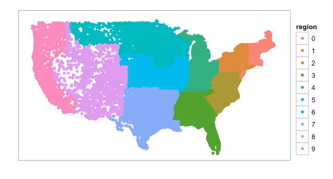
Now we wouldn’t be R users if we didn’t try to do something with data, even if it’s just a lookup table of zip codes. So let’s take a look at how they’re distributed by first digit:

library(zipcode)
library(ggplot2)

data(zipcode)
zipcode$region = substr(zipcode$zip, 1, 1)

g = ggplot(data=zipcode) + geom_point(aes(x=longitude, y=latitude, colour=region))

# simplify display and limit to the "lower 48"
g = g + theme_bw() + scale_x_continuous(limits = c(-125,-66), breaks = NA)
g = g + scale_y_continuous(limits = c(25,50), breaks = NA)

# don't need axis labels
g = g + labs(x=NULL, y=NULL)

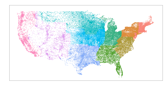
If we make the points smaller, cities and interstates are clearly visible, at least once you leave the Northeast Megalopolis:

spssread.pl: a Perl script to parse SPSS SAV file metadata

I have been spending some time trying to figure out why R’s read.spss() function won’t read Qualtrics-generated SPSS SAV files. (Qualtrics is a very nice online survey system which we have been using with one of our partners.)

I have to admit that I have no interest in the structure of SPSS files (or most others, for that matter), so I was very glad to find Scott Czepiel’s spssread.pl Perl script to parse and display metadata.

So far I can tell that R’s read.spss()/code> is croaking on null characters (as in ASCII 0) at the end of variable names. What was puzzling is that the open source PSPP seems to read these Qualtrics files just fine and the read.spss() code was originally based on PSPP.

To read these files from R, I have been reading them into PSPP first and saving new copies.

Thanks to spssread.pl, I can now see that PSPP doesn't like these variable names either. But instead of croaking, PSPP simply assigns new variable names as spssread.pl -r shows:

$ ./spssread.pl -r qualtrics_short.sav 
Name	Type	Label
A_1	String (20)	ResponseID  
A_2	String (20)	ResponseSet 
A_3	String (255)	Name
A_4	String (255)	ExternalDataReference   
A_5	String (255)	Email   
A_6	String (255)	IPAddress   
A_7	String (255)	StartDate   
A_8	String (255)	EndDate 
A_9	Numeric	Finished
A_10	Numeric	Many airlines are involved in a continui
A_11	Numeric	Please check which applies to this trip.
A_12	Numeric	About how full was your cabin of the air
A_13	Numeric	What was the primary purpose of this fli
A_14	Numeric	Who made the decision regarding the airp
A_15	Numeric	Please divide 100 points among the five -Schedule convenience   
A_16	Numeric	Please divide 100 points among the five -Preference for airline 
A_17	Numeric	Please divide 100 points among the five -Frequent flyer/Mileage program 
A_18	Numeric	Please divide 100 points among the five -Ticket price   
A_19	Numeric	Please divide 100 points among the five -Company policy 
A_20	Numeric	How close to the scheduled departure tim
A_21	Numeric	Please rate the services you received fr-Speed in getting through to Agent  
A_22	Numeric	Please rate the services you received fr-Helpfulness of Agent   
A_23	Numeric	Please rate the services you received fr-Courtesy of Reservation Agent  
A_24	Numeric	Please rate the services you received fr-Accuracy of flight information 
A_25	Numeric	Please rate the services you received fr-Accuracy of fare information   
A_26	Numeric	Please rate the services you received fr-Value for the money
A_27	Numeric	Please rate the services you received fr-Overall rating of the flight   
A_28	String (255)	Including this trip how many air trips fBusiness
A_29	String (255)	Including this trip how many air trips fPleasure
A_30	Numeric	For classification purposes are you...  
A_31	String (255)	Approximate age:
A_32	Numeric	Occupation  
A_33	Numeric	Approximately how many people are employ
A_34	String (255)	City and state of residence:
A_35	Numeric	THANK YOU FOR YOUR COOPERATION. 

$ ./spssread.pl -r pspp_short.sav 
Name	Type	Label
V1      	String (20)	ResponseID  
V2      	String (20)	ResponseSet 
V3      	String (255)	Name
V4      	String (255)	ExternalDataReference   
V5      	String (255)	Email   
V6      	String (255)	IPAddress   
V7      	String (255)	StartDate   
V8      	String (255)	EndDate 
V9      	Numeric	Finished
A22777  	Numeric	Many airlines are involved in a continui
A22778  	Numeric	Please check which applies to this trip.
A22779  	Numeric	About how full was your cabin of the air
A22780  	Numeric	What was the primary purpose of this fli
A22781  	Numeric	Who made the decision regarding the airp
A22782_1	Numeric	Please divide 100 points among the five -Schedule convenience   
A22782_2	Numeric	Please divide 100 points among the five -Preference for airline 
A22782_3	Numeric	Please divide 100 points among the five -Frequent flyer/Mileage program 
A22782_4	Numeric	Please divide 100 points among the five -Ticket price   
A22782_5	Numeric	Please divide 100 points among the five -Company policy 
A22783  	Numeric	How close to the scheduled departure tim
A_21    	Numeric	Please rate the services you received fr-Speed in getting through to Agent  
A_22    	Numeric	Please rate the services you received fr-Helpfulness of Agent   
A_23    	Numeric	Please rate the services you received fr-Courtesy of Reservation Agent  
A_24    	Numeric	Please rate the services you received fr-Accuracy of flight information 
A_25    	Numeric	Please rate the services you received fr-Accuracy of fare information   
A_26    	Numeric	Please rate the services you received fr-Value for the money
A_27    	Numeric	Please rate the services you received fr-Overall rating of the flight   
A22823_0	String (255)	Including this trip how many air trips fBusiness
A22823_1	String (255)	Including this trip how many air trips fPleasure
A22825  	Numeric	For classification purposes are you...  
A22826_0	String (255)	Approximate age:
A22827  	Numeric	Occupation  
A22828  	Numeric	Approximately how many people are employ
A22829_0	String (255)	City and state of residence:
Q16     	Numeric	THANK YOU FOR YOUR COOPERATION. 

File header information can be displayed with spssread.pl -h:

$ ./spssread.pl -h qualtrics_short.sav 

Record type         $FL2
Product name        @(#) SPSS DATA FILE PHP Writer (c) Qualtrics - 0.9.0        
Layout code         2
Case Size           349
Compression         1
Weight index        0
Number of cases     -1
Bias                100.000000
Creation date       21 Jul 10
Creation time       10:28:27
File label                                                                          

$ ./spssread.pl -h pspp_short.sav 

Record type         $FL2
Product name        @(#) SPSS DATA FILE GNU pspp 0.7.6-g55e6e7 - i386-apple-darw
Layout code         2
Case Size           349
Compression         1
Weight index        0
Number of cases     1
Bias                100.000000
Creation date       15 Dec 10
Creation time       12:57:31
File label                                                                          

Thanks, Scott. spssread.pl sure beats the heck out of some quality time with od and the SAV file format docs!

How to fix PSPP’s psppire crashing right after launch (Mac OS 10.5.8)

I installed PSPP from MacPorts on Mac OS X 10.5.8. When I launch the psppire GUI, it displays the splash screen, opens its main window, then crashes a couple of seconds later:

$ /opt/local/bin/psppire
Xlib:  extension "RANDR" missing on display "/tmp/launch-T7iqdy/:0".
(psppire:64632): Gtk-WARNING **: Could not find the icon 'application-x-spss-sav'.
The 'hicolor' theme was not found either, perhaps you need to install it.
You can get a copy from:
http://icon-theme.freedesktop.org/releases
**
Gtk:ERROR:gtkrecentmanager.c:1942:get_icon_fallback: assertion failed: (retval != NULL)
Abort trap

Upgrading to the pspp-devel beta version didn’t help.

Solution

Google found a recent ticket and discussion for the same problem with “MyPaint” installed from MacPorts. Maybe it’s a generic problem caused by a change to MacPorts. Dunno, but the same workaround fixed PSPP for me:

  1. Install gnome-icon-theme via MacPorts
  2. Create ~/.gtkrc-2.0 with the line

    gtk-icon-theme-name = "gnome"

Ta-da:

$ /opt/local/bin/psppire
Xlib: extension "RANDR" missing on display "/tmp/launch-T7iqdy/:0".

PSPP screenshot

The “RANDR” warning doesn’t seem to matter.

Posted in Tips. Tags: , , . Leave a Comment »